PivotTables

One way to increase the usability of your aPriori spreadsheet reports is to enhance your Excel template files with PivotTables®. This is not an aPriori-specific topic, so this section does not go into depth. You should go to Excel documentation for general Pivot Table information. But this section gives you an overview as to how to use Pivot Tables with aPriori data.

When to use PivotTables

Consider using PivotTables when you want to create relatively simple tabular or graphical views of your aPriori data. You can also use PivotTables to filter out a certain data point (or points) from the output data worksheet.

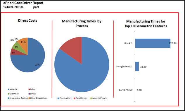
Define a PivotTable Template

1. Create and install a spreadsheet report.
2. Run the spreadsheet report on actual data.
3. Open the output .xls file and use the Insert>PivotTable>PivotTable and/or PivotChart feature to define the range of data you want to use from the output tab.
4. Refer to Excel on-line help for details about defining your PivotTable and PivotChart.
5. Click PivotTable Options > Data and ensure that “Refresh data when opening the file is checked.
6. Remove the output tab and ReportSummarySheet tabs. This is now your template.
7. Update the template path of your watchpoints.xml file to reference the new Excel template.
8. Install and run the report.

Use a PivotTable to Filter out Data

To filter the PivotTable to display the information you want, you must select a path that, when used, only displays the information you want. For example,

1. Follow Steps 1 - 3 in “To Define a PivotTable Template”.

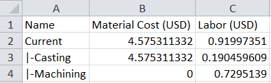
2. In this case, you want to display the labor cost for the casting process in a report. Here is the data that is output when the report is run:

   

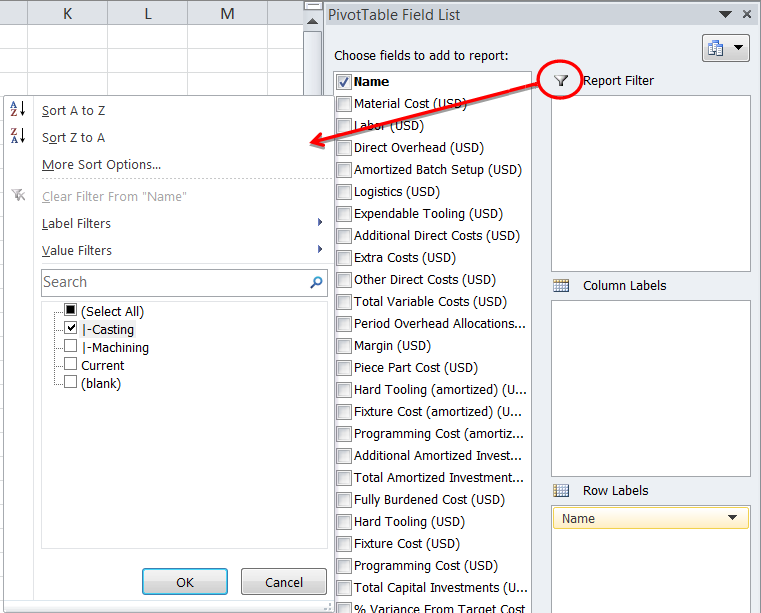
3. When you create the PivotTable Insert > PivotTable > PivotTable, you can start to create the path to display the information you want. The quickest path to display labor cost for casting is to first select the checkbox for Name in the PivotTable Field List and to filter the Name column to show only information for Casting:

   

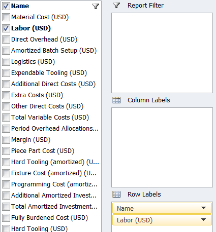
4. Select the Labor (USD) box to show the labor cost for the Casting process:

   

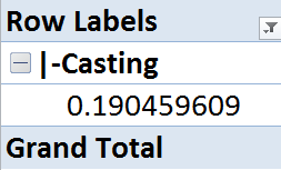
5. of the PivotTable should look like the following. The report template can then read this cell for every time the report is run to then always show the labor cost for the casting process.

   

Using Filters

This same method can be used for data outputs that require as many filters as you need to get only the information that you want to show. The following is an example of using more filters.

Task

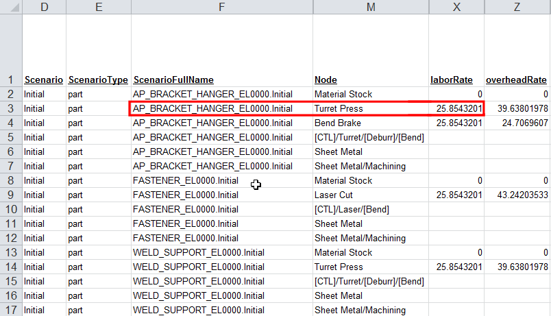
To display Labor Rate for the turret press process for the part name “AP_BRACKET_HANGER_EL0000.Initial”.

• View the red box that shows the path the PivotTable should take.

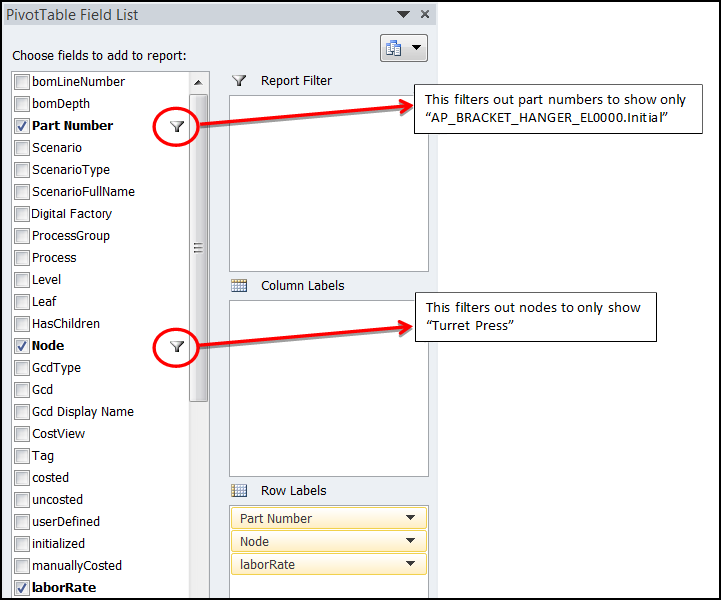
• Select the three checkboxes, and you apply the two filters; the PivotTable displays only the labor rate for the turret press node for the selected part.

• After the three boxes and the two filters, the PivotTable displays only the labor rate for the turret press node for the selected part.